9. Causal Effects and Adjusted Marginal Contrasts (RMST)

Moving Beyond the Hazard Ratio

In clinical trials and observational studies, researchers often wish to compare survival outcomes between two groups. Historically, this is answered using the Hazard Ratio (HR) from a Cox Proportional Hazards model. However, the HR is non-collapsible—meaning the omission of unmeasured covariates will mathematically bias the effect toward the null—and strictly relies on the proportional hazards assumption. If survival curves cross, the HR becomes mathematically invalid.

SuperSurv solves this by evaluating group differences on the absolute time scale using the Restricted Mean Survival Time (RMST) via G-computation (Standardization) on top of our Ensemble Super Learner.

RMST calculates the area under the survival curve up to a specific time horizon, $\tau$ . By comparing the expected RMST if everyone in the dataset belonged to Group 1 versus if everyone belonged to Group 0, we obtain a robust, absolute measure of the difference:

$\Delta \text{RMST} = E[Y(1)] - E[Y(0)] = \text{RMST}_{\text{Group 1}}(\tau) - \text{RMST}_{\text{Group 0}}(\tau)$

Philosophy: “Causal Effect” vs. “Marginal Contrast”

How you interpret this $\Delta \text{RMST}$ depends entirely on the nature of your exposure variable. The math of G-computation is identical for both, but the statistical terminology must be used responsibly.

Causal Average Treatment Effect (ATE): You can claim a Causal Effect if your variable is a manipulable intervention. Examples include administering a drug, performing a surgery, or applying a policy.
- Interpretation: “Administering this drug causally adds an average of 4.2 months of life over a 5-year period compared to the placebo.”
Adjusted Marginal Contrast: You must claim an Adjusted Marginal Contrast if your variable is an immutable trait or biological group. Examples include biological sex, race, or a genetic biomarker. Because you cannot “causally” intervene to change someone’s genetics, we are simply comparing two groups while rigorously adjusting for all other confounding variables.
- Interpretation: “After adjusting for all baseline clinical covariates, the presence of this biomarker is marginally associated with 4.2 additional months of survival over a 5-year period.”

Estimating the Effect with `SuperSurv`

Let’s demonstrate this using the built-in metabric dataset. We will evaluate the effect of the binary biomarker x4 (1 = present, 0 = absent). Because x4 is a biomarker, we will interpret the result as an Adjusted Marginal Contrast.

library(SuperSurv)
set.seed(123)

# Load built-in data
data("metabric", package = "SuperSurv")

# Define predictors and time grid
X <- metabric[, grep("^x", names(metabric))]
new.times <- seq(10, 150, by = 10)

1. Train the Super Learner

First, train the ensemble. We must set control = list(saveFitLibrary = TRUE) so the models are saved for the G-computation prediction phase.

fit <- SuperSurv(
  time = metabric$duration,
  event = metabric$event,
  X = X,
  newdata = X,
  new.times = new.times,
  event.library = c("surv.coxph", "surv.rfsrc"),
  cens.library = c("surv.coxph"),
  control = list(saveFitLibrary = TRUE) 
)

2. Calculate the Counterfactual RMST

We use the estimate_causal_rmst() function. This forces the biomarker x4 to 1 for all patients, predicts their survival curves, and calculates the RMST, then repeats with x4 forced to 0.

# Estimate the adjusted difference up to tau = 100 months
results <- estimate_marginal_rmst(
  fit = fit, 
  data = metabric, 
  trt_col = "x4", 
  times = new.times, 
  tau = 100
)

print(results$ATE_RMST)

Interpretation: If the resulting $\Delta$ RMST value is 4.2, we interpret this marginal contrast as: “After adjusting for complex baseline covariates via the Super Learner ensemble, patients with biomarker x4 live an average of 4.2 months longer over a 100-month horizon compared to those without the biomarker.”

3. Visualizing the Effect Over Time

The difference between groups might be near zero early on but substantial later. We can visualize how the $\Delta$ RMST evolves across different time horizons using plot_causal_rmst_curve().

# Plot the Delta RMST across a sequence of tau values
tau_grid <- seq(20, 140, by = 20)
plot_marginal_rmst_curve(
  fit = fit, 
  data = metabric, 
  trt_col = "x4", 
  times = new.times, 
  tau_seq = tau_grid
)

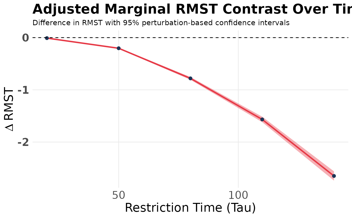
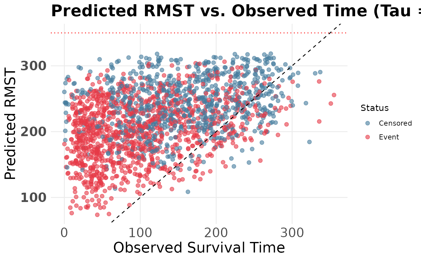
4. Diagnostic: Predicted RMST vs. Observed Time

To evaluate how well our model’s restricted expectations align with reality, we can plot the predicted RMST for the observed data against their true survival times. Patients who experienced the event should lie close to the diagonal line up to $\tau$ .

plot_rmst_vs_obs(
  fit = fit, 
  data = metabric, 
  time_col = "duration", 
  event_col = "event", 
  times = new.times, 
  tau = 350
)