08. Interpreting the Black Box with SHAP & survex
Source:vignettes/shap-explanations.Rmd
shap-explanations.RmdIntroduction
Machine learning models are notoriously criticized as “black boxes.” While they often achieve superior predictive performance, clinicians need to know why a model is making a specific prediction.
SuperSurv solves this using SHAP (SHapley
Additive exPlanations). Because Shapley values possess the
mathematical property of linearity, SuperSurv can calculate
the SHAP values for every active base learner and seamlessly combine
them using the meta-learner’s weights.
This tutorial covers Global feature importance, Local (patient-level)
explanations, and Time-Dependent survival analysis using the
survex package.
1. Setup and Model Fitting
Let’s train a diverse Super Learner on our metabric
dataset.
library(SuperSurv)
library(survival)

data("metabric", package = "SuperSurv")
set.seed(42)

train_idx <- sample(1:nrow(metabric), 0.7 * nrow(metabric))
train <- metabric[train_idx, ]
test  <- metabric[-train_idx, ]

X_tr <- train[, grep("^x", names(metabric))]
X_te <- test[, grep("^x", names(metabric))]
new.times <- seq(50, 200, by = 25)

my_library <- c("surv.coxph", "surv.weibull", "surv.rfsrc")

fit_sl <- SuperSurv(
  time = train$duration,
  event = train$event,
  X = X_tr,
  newdata = X_te,
  new.times = new.times,
  event.library = my_library,
  cens.library = c("surv.coxph"),
  verbose = FALSE,
  selection = "ensemble",
  nFolds = 3
)
2. Global Explanations (Kernel SHAP)
To calculate static risk SHAP values, we need an
X_explain dataset (the patients we want to explain) and an
X_background dataset (a reference population used to
calculate the baseline average risk).
# Explain the first 50 test patients using 100 training patients as the background
X_explain_subset <- X_te[1:50, ]
X_background_subset <- X_tr[1:100, ]

# Calculate weighted Ensemble SHAP values using Kernel SHAP
shap_vals <- explain_kernel(
  model = fit_sl,
  X_explain = X_explain_subset,
  X_background = X_background_subset,
  nsim = 20
)
Global Importance Bar Plot
Which features drive the ensemble’s mortality risk predictions across the entire cohort?
plot_global_importance(shap_vals, top_n = 5)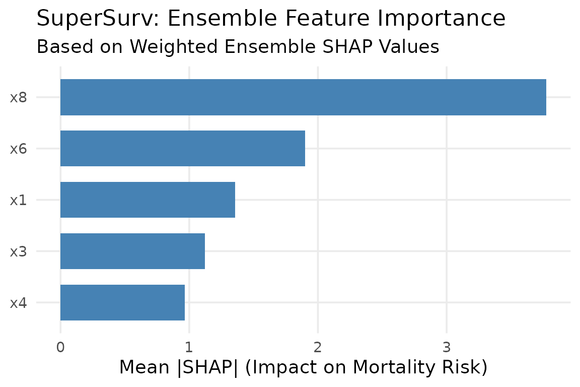
SHAP Beeswarm Summary Plot
The beeswarm plot is the gold standard for SHAP. It shows both the magnitude of a feature’s impact and the direction of its effect.
plot_beeswarm(shap_vals, data = X_explain_subset, top_n = 5)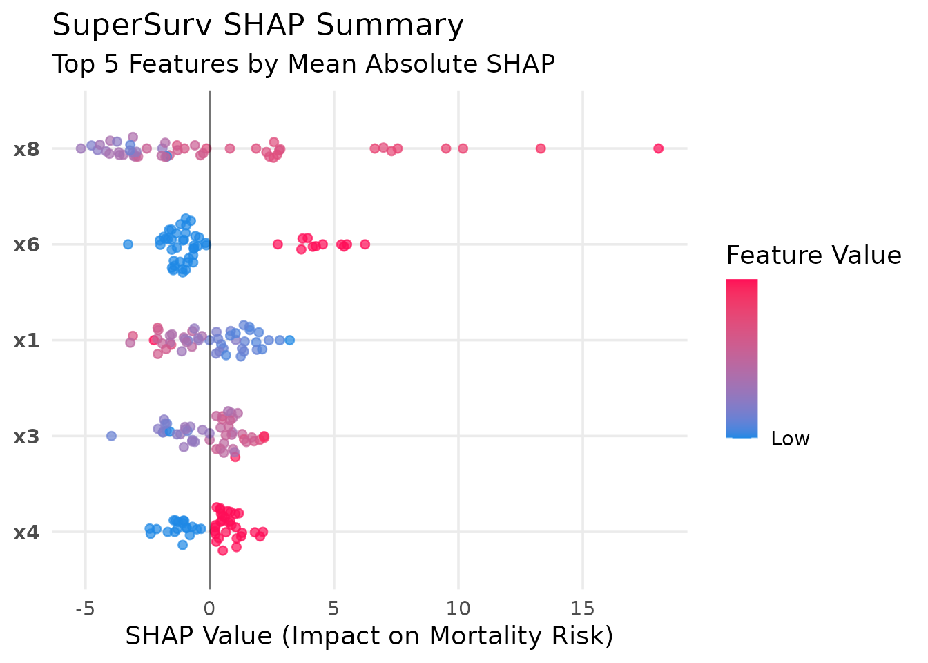 Interpretation: A red dot (high feature value) on the right side of
the vertical zero-line indicates that higher values of this biomarker
increase mortality risk.
Interpretation: A red dot (high feature value) on the right side of
the vertical zero-line indicates that higher values of this biomarker
increase mortality risk.
3. Local (Patient-Level) Explanations
In precision medicine, we often need to explain why a specific patient has a high risk score. The Waterfall plot breaks down the exact algorithmic logic for an individual.
# Explain Patient #1 from our test subset
plot_patient_waterfall(shap_vals, patient_index = 1, top_n = 5)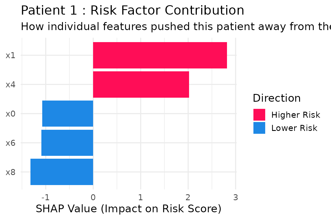
4. Feature Dependence Plots
Does a specific biomarker have a linear or non-linear relationship with mortality risk?
plot_dependence(shap_vals, data = X_explain_subset, feature_name = "x0")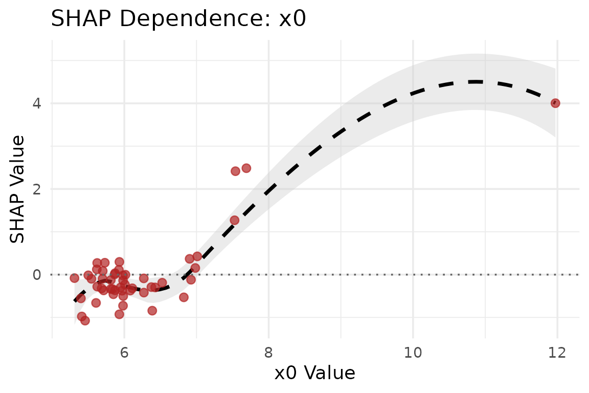
5. Patient Risk Trajectories (Survival Heatmap)
We can visualize patient trajectories over time using a survival
heatmap generated directly from SuperSurv predictions.
# Plot the survival trajectories for the first 50 test patients
plot_survival_heatmap(fit_sl, newdata = X_explain_subset, times = new.times)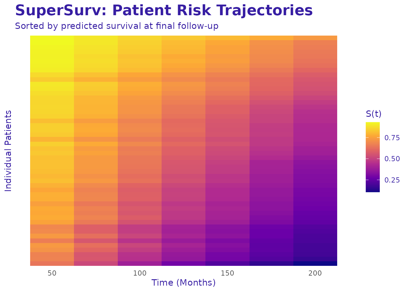 Interpretation: Patients at the top experience rapid drops in
survival probability (high risk), while patients at the bottom maintain
high survival probabilities.
Interpretation: Patients at the top experience rapid drops in
survival probability (high risk), while patients at the bottom maintain
high survival probabilities.
6. Time-Dependent Explanations (survex
Integration)
Traditional SHAP looks at an overall “risk score,” but survival analysis is fundamentally about time. A feature might be highly predictive of early mortality (Time = 50) but irrelevant for long-term survival (Time = 200).
SuperSurv natively bridges to the survex
package to evaluate dynamic feature importance across the entire
survival curve
.
library(survex)

# 1. Create the true survival object for the explanation subset
y_explain <- survival::Surv(test$duration[1:50], test$event[1:50])

# 2. Build the survex explainer using our custom function
surv_explainer <- explain_survex(
  model = fit_sl,
  data = X_explain_subset,
  y = y_explain,
  times = new.times
)
Once the explainer is created, you have full access to the
survex ecosystem. Let’s look at three powerful
time-dependent visualizations.
A. Dynamic Feature Importance
Which features are driving the model’s predictions at different clinical milestones?
# Calculate time-dependent model parts (permutation feature importance)
time_importance <- model_parts(surv_explainer)
# Plot the dynamic importance over time
plot(time_importance)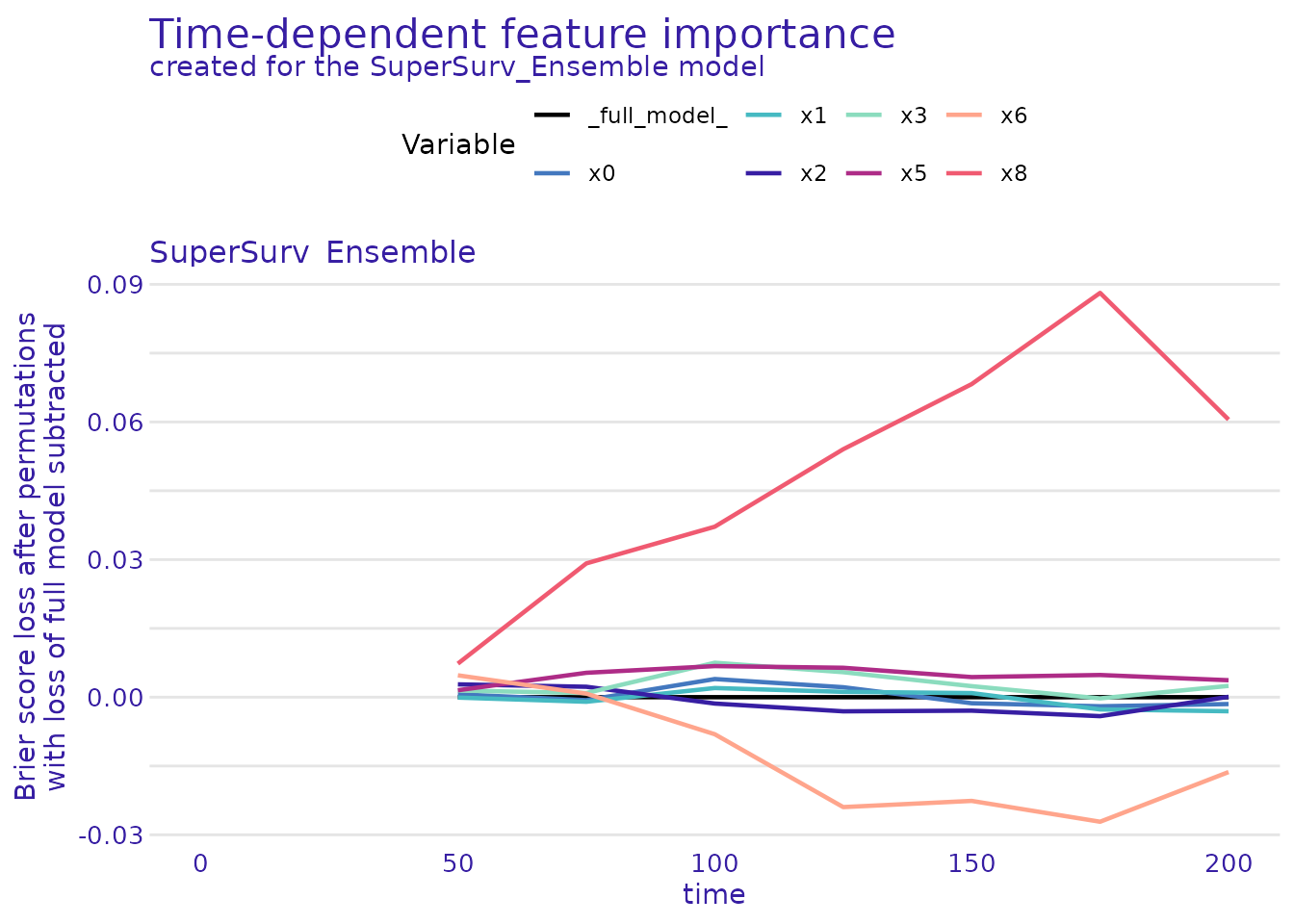 Interpretation: If a feature’s curve rises over time, it means that
biomarker becomes more critical for predicting long-term
survival.
Interpretation: If a feature’s curve rises over time, it means that
biomarker becomes more critical for predicting long-term
survival.
B. Time-Dependent Partial Dependence Profiles
How does the value of a specific continuous feature (e.g.,
x0) change the average survival probability over time?
# Calculate the partial dependence profile for feature 'x0'
pdp_time <- model_profile(surv_explainer, variables = "x0")
plot(pdp_time)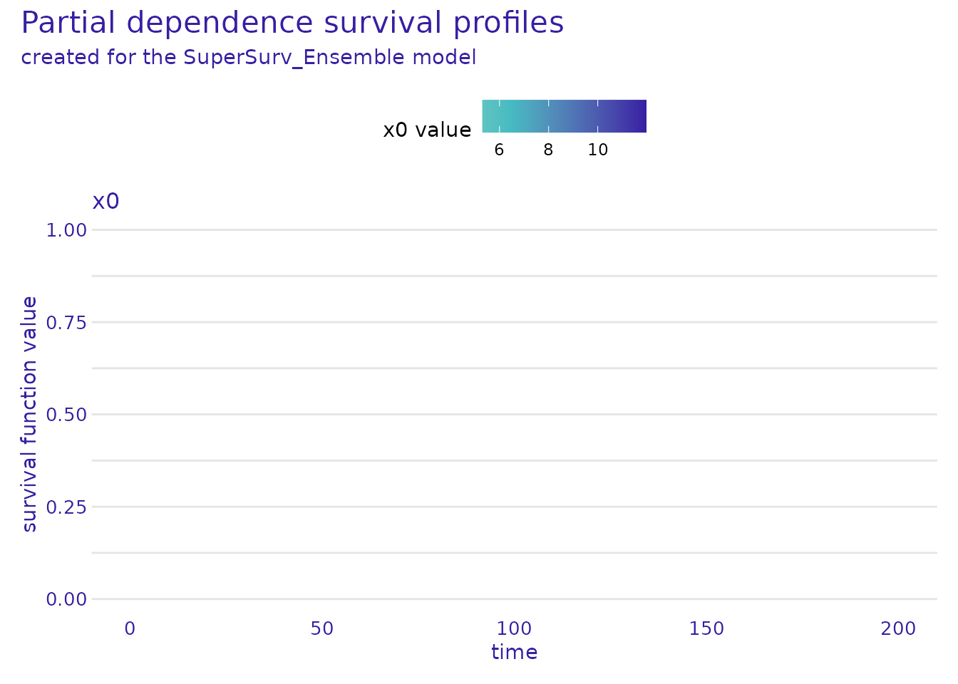 Interpretation: This generates a 3D-like profile showing how
different values of
Interpretation: This generates a 3D-like profile showing how
different values of x0 shift the entire survival
curve.
C. SurvSHAP(t): Local Explanations Over Time
Just like the Waterfall plot explains a static risk score, SurvSHAP(t) explains exactly how a specific patient’s features pushed their survival probability up or down at every single time point.
# Explain Patient #1 over time
patient_1_data <- X_explain_subset[1, , drop = FALSE]
# Calculate SurvSHAP(t)
survshap_t <- predict_parts(surv_explainer, new_observation = patient_1_data, type = "survshap")
plot(survshap_t)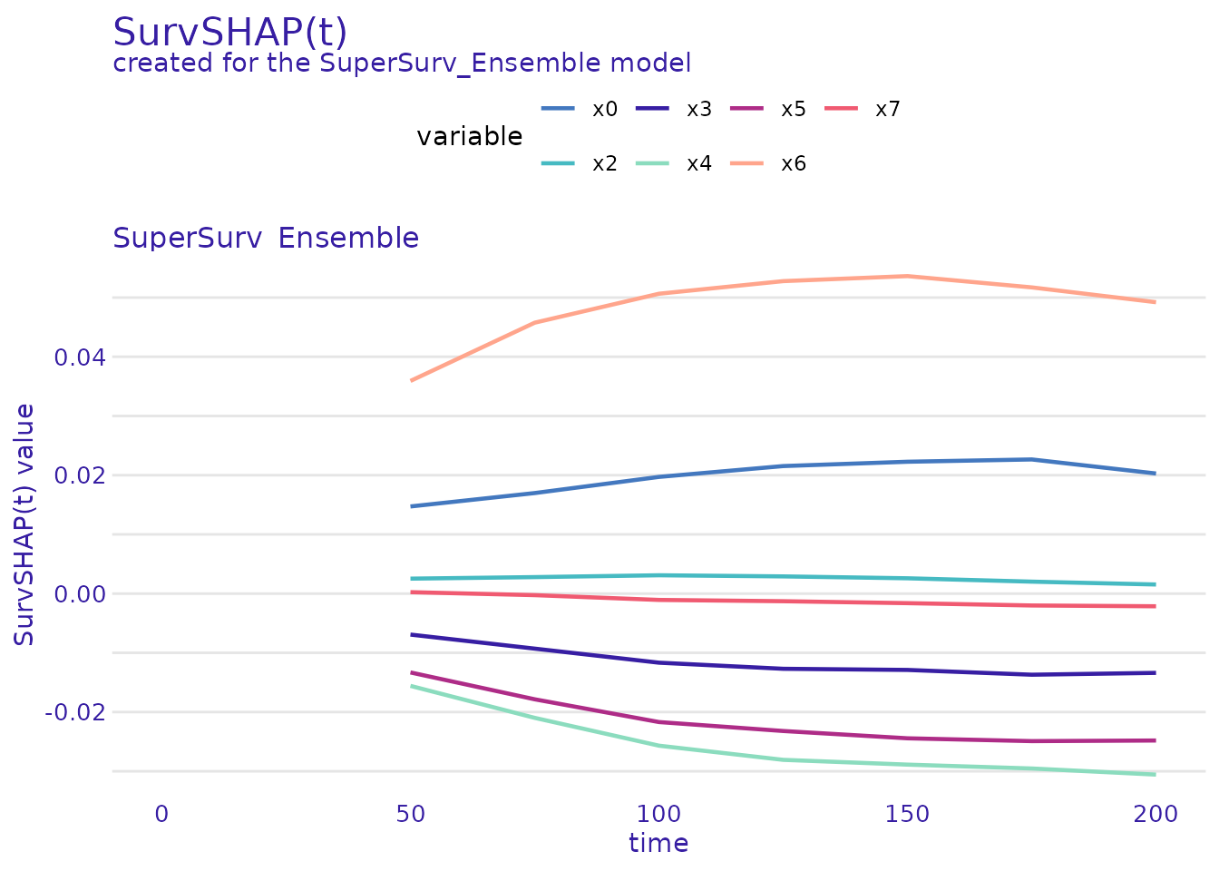 Interpretation: The solid black line is the model’s average survival
curve. The colored areas show how Patient 1’s specific covariates (like
their specific age or tumor grade) dragged their personal survival curve
above or below the average over time.
Interpretation: The solid black line is the model’s average survival
curve. The colored areas show how Patient 1’s specific covariates (like
their specific age or tumor grade) dragged their personal survival curve
above or below the average over time.
D. Ecosystem Compatibility: Global Model Performance
Because explain_survex() creates a standard explainer
object, you aren’t just limited to SHAP values. You can utilize the
entire survex ecosystem, including their built-in
performance metrics.
While SuperSurv provides its own comprehensive
benchmarking suite (plot_benchmark), you can easily
cross-validate your ensemble’s Time-Dependent Brier Score and AUC using
survex’s native functions:
# Calculate time-dependent performance metrics via survex
survex_perf <- model_performance(surv_explainer)
# Plot the Brier score and AUC curves
plot(survex_perf)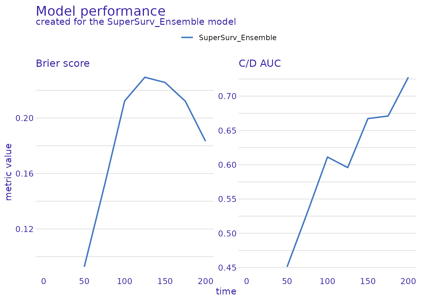 Note: The Brier score should ideally stay as low as possible over
time, while the AUC should remain high. This serves as an excellent
independent validation of the results generated by
Note: The Brier score should ideally stay as low as possible over
time, while the AUC should remain high. This serves as an excellent
independent validation of the results generated by
SuperSurv’s native eval_summary()!
By utilizing these tools, SuperSurv ensures that your
advanced machine learning ensembles remain completely transparent,
dynamically interpretable, and ready for clinical deployment.